Image Filtering and Noise Reduction

Introduction

In this blog, we will look at image filtering which is the first and most important pre-processing step that almost all image processing applications demand. The content is structured as following:

1. In the context of noisy gray-scale images, we will explore the mathematics of convolution and three of the most widely used noise reduction algorithms.
2. Next, we will analyze the pros and cons of each algorithm and measure their effectiveness by applying them to a test case.
3. We will hence conclude by the defining parameters to look for when choosing between these three algorithms.

Image Filtering

At its core, an image filtering algorithm generates an output pixel by observing the neighborhood of a given input pixel in an image. This operation, if linear, calculates the output pixel value by linearly combining, in accordance with some algorithm rule, the values of a set of pixels in proximity of the corresponding input pixel through their relative positions. This process can be used to enhance or reduce certain features of image while preserving the other features. Convolution is a form of linear filtering which is mathematically explained in the following section.

Convolution

While dealing with images, we are basically dealing with matrices. For gray-scale images, where each pixel represents the intensity of light at that point, the matrix is 2-dimensional. Convolution is a prominent concept used in a variety of image processing algorithms. Before diving deep into algorithms, it is vital we understand convolution precisely.

Kernel is a matrix with predefined values at each index. The result of convolution is a transformed image of the original image.

Let us assume we have defined a 3-by-3 kernel, к =

a         b      c

d        e        f

g        h       i

The first step of convolution is to flip the columns and rows of the kernel matrix. Let us represent the flipped matrix of к by к_f =

i         h         g

f          e        d

c         b        a

Note that for symmetric kernel, flipping rows and columns returns the original kernel matrix.

The next step is to slide this flipped matrix through the input image by placing the center of кf over each image pixel. When we do this, we replace the pixel value by multiplying kernel elements with pixel values directly below them and then taking the sum. If at a given instance, the following was the image matrix below the sliding к_f, when its center was placed over the image coordinates (x, y), denoted by ɪ_m =

p1       p2      p3

p4       p5      p6

p7       p8       p9

  Then in the transformed image, at the pixel position (x, y) the pixel value is =

i * p₁   + h * p₂  + g * p₃  + f * p₄  + e * p₅  + d * p₆  + c * p₇  + b * p₈  + a * p₉

From the above equation, we can derive that each image pixel value is replaced by the weighted sum of neighboring pixels with weights defined by flipped kernel elements over them. If ɪ denotes the input image matrix, then the transformed or output image obtained by convolving with к is denoted as =

Noise Reduction algorithms

Now that we have understood convolution, let us look at image filtering and some of the most commonly used image filtering methods.

A digital image often contains noise. Noise introduces erroneous pixel values. Image filtering is the process of removing these errors. Convolving a noisy image with an appropriate kernel practically nullifies the noise.

Let us have a look at the different image filtering methods in the subsequent paragraphs. For all the below filters, let the kernel size be K_height*K_width.

Normalized Box Filter:

If all the elements of a kernel are given unit values, convolving it with image would mean replacing the pixel values with the sum of its neighbor in K_height*K_width window. If each element in kernel is now divided by the kernel size, then the sum of all elements will be 1, the normalized form.  Such a convolution would result in pixel values being replaced by mean or arithmetic average of neighboring pixels in the K_height*K_width window. This effect can be used to achieve smoothness in images. Taking average would mean reduction in sudden changes in intensity values between neighboring pixels.

Normalized box filter of size 3*3 =

Gaussian Filter:

A Gaussian equation is of the following form:

 ————————————— eq(1)

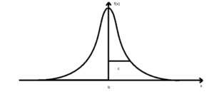
In the above diagram, we can see that the values near the reference point are more significant. This same Gaussian distribution is achieved in a 2-dimensional kernel with the reference point being matrix center. As opposed to Normalized Box filter which gives equal weight to all neighboring pixels, a Gaussian kernel gives more weight to pixels near the current pixel and much lesser weight to distant pixels when calculating sum.

Bilateral Filter:

While Gaussian filter gives us more control and accurate results than box filter, both the filters err when taking weighted sum of edge pixels. Both of the filters smoothen the edge pixels, thereby diminishing the intensity variant. Bilateral filter overcomes this shortcoming.

While Gaussian filter assigns weight to neighbors based only on their distance from the current pixel, bilateral filter brings intensity to the picture. Now the shape of the Gaussian function is determined solely based on or the standard deviation. Let us assume the following symbols:

• _Çd = standard deviation of Gaussian used for spatial filtering
• _ci = standard deviation of Gaussian used for intensity filtering
• α = a pixel in the input image
• I(α) = intensity at pixel α
• I_f (α) = value at pixel α after taking weighted sum of neighboring pixels as per the convolving kernel
• || α_r – α_s || = Euclidian distance between the two pixels α_r and α_s
• ϴ = window centered at pixel α, the size of window is the size of the kernel
• N = normalization factor for the kernel

If we were taking only Gaussian filter, then the calculated value at pixel α will be:

——————————eq(2)

We can again observe from the above equation that the weight given to I(α_n) – intensity at a neighbor pixel α_n simply depends on its Euclidian distance from the current pixel α in the sum. The closer a neighbor pixel is to reference (current) pixel, the more weight it gets.

Let’s see what happens when we change the above equation to one as below:

————————————–eq(3)

Now the weight given to I(α_n) – intensity at a neighbor pixel α_n also depends on its intensity difference when compared with the intensity at pixel α – I(α). The closer a neighbor pixel is to reference (current) pixel, the more weight it gets. But additionally, it also needs to be close in terms of intensity to reference pixel. Even if a neighbor pixel is close but differs a lot when intensities are compared to reference pixel, it will be given much less weight.

Now let’s see what happens when during convolution, we are at an edge pixel as highlighted below:

Eq(2) gives the same weight to pixel value at the immediate left of edge pixel as the weight given to immediate right. This weight distribution will blur the difference made apparent by this edge pixel.

Eq(3) however, observes that there is a considerable difference in intensities for the pixel at immediate left of edge pixel. As we know the behavior of Gaussian, the larger the difference from reference point, the smaller the weight it generates. Here the reference point is the intensity at edge pixel. Hence it gives more weight to pixel at right and much lesser weight to pixel at left in comparison. Hence the edge is preserved.

Analysis

Let us analyze each of the above three algorithms as image filtering operations via a test case.

Problem Statement:

When we think of filtering in images, we always define image features that we want to modify and those that we want to preserve. Let us observe the following original image with no noise and surface plot of one of its patch.

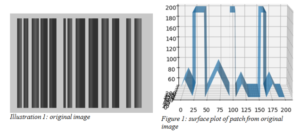
Following are the observations:

1. The image consists of uniform whitish background embedded with blackish bars. In fact for the above system, it is constrained that intensity of any pixel within a bar and that of any background pixel exceeds a minimum difference δ.
2. Another thing of note portrayed by the surface plot is that each black bar has a vertical line where the intensity peaks within.
3. The width of the bars and peak pixels within them seem to be varying discretely. This is the encoded information that the bars represent.

We can now define the features and strict constraints on them that we are interested in:

1. edge pixels that form the boundary between bars and background can easily be labeled by detecting pixels whose intensity difference with immediate neighboring pixel exceeds δ.
2. peak pixels are ensured if we strictly detect that consecutive two adjacent pixels on either side have a decreasing trend in intensity. Namely if p1, p2, p3, p4, p5 are consecutive pixels horizontally, ensuring I(p2) < I(p3) & I(p1) < I(p2) & I(p4) < I(p3) & I(p5) < I(p4) should strictly ensure p3 is a peak pixel.

Applying the above two constraints on the given image, the following feature image is generated.

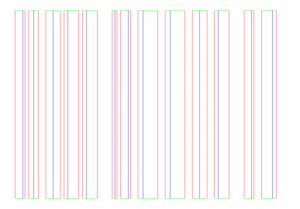
Illustration 2: features of original image

An edge is always normal to intensity variation. Thereby,

• Red pixels are edge pixels with horizontal intensity difference > δ
• Green pixels are edge pixel with vertical intensity difference > δ
• Blue pixels are peak pixels

Entrance of the Enemy:

Let us introduce some reality into our ideal world till now – noise. Let us model the real world noise as normally distributed in accordance with the Central Limit Theorem. We are using the python opencv function randn to generate this noise. When added to the above original image, it has the following effect:

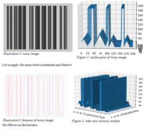
• The surface is not smooth anymore and has numerous distorted spikes
• Peaks seem to be the most affected by noise

Performance Measure:

We want to measure how closely we have retrieved the original image features after applying a noise removal algorithm. If after applying the same strict constraints on a filtered image, red, blue or green pixels are detected, we want to measure how many of them have preserved their original position respectively. True positives and false positives are indicators of that. Equally, we also want to measure how much of our expectations are met. Below are the four performance metrics for peak pixels (blue):

Positive indicators:

• true positives: in percentage of all the blue pixels detected, how many were at their original (correct) location
• expectations met: in percentage from all the blue pixels from original image, how many were detected in the current image

Negative indicators:

• false positives: complementary of true positives, in percentage of all the blue pixels detected, how many were at different (false) location
• expectations failed: complementary of expectations met, in percentage from all the blue pixels from original image, how many were not detected in the current image

Similar metrics apply for red and green pixels.

State of noisy image:

The result for edge pixels is perfect. Though noise has distorted the image, it is not strong enough to alter edge pixel intensities so much that neighbor difference falls below δ, as apparent from figure 2. But the peaks have taken the worst hit. Of all the pixels that were detected, just 31.86% of them were true peaks.  Moreover only 34.06% of our expectations were met. 65.94% of true peaks were never detected. Let us address this serious concern by applying noise reduction algorithms one by one and choose the best one.

Apply Normalized Box Filter:

The box filter algorithm only exposes one parameter that we can control – the kernel dimension which can only be odd numbered. Keeping the kernel size as 3*3 has very little effect on the image. We try with kernel size of 5, which most literature recommends. We will find out the reason soon.

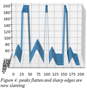
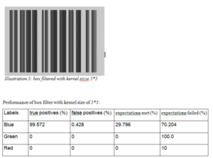
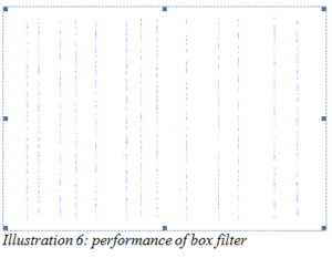
Peak pixels are now truly positive. 99.57% of all peaks detected are indeed true peaks. But the reality is only 29.80% of expected true peaks are detected. More drastic is the effect on edge pixels. Not a single red or green pixels are detected which means an expectation failure of 100%.

Figure 4 clearly explains the reason. Though the surface has smoothed and noise has been virtually eliminated, taking the average of neighbor pixels has resulted in peaks becoming flatter and sharp edges demonstrating slanting behavior.

Increasing the kernel size increases the computational cost while further flattening out peaks and diminishing edges.

Apply Gaussian Filter:

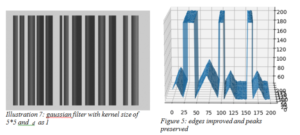
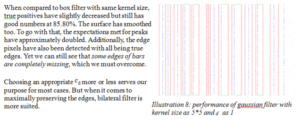
Overcoming the shortcoming of box filter, Gaussian filter distributes weight among its neighbor pixels depending on parameter –c _d, the standard deviation in space. Keeping the kernel size same as 5*5 and varying c _d, we achieve the best result with standard deviation as 1.

Apply Bilateral Filter:

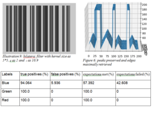
Besides kernel size and c_d, bilateral filter exposes an additional parameter to control performance c- _I, the standard deviation in intensity domain. Keeping the same kernel size as 5*5, we obtain the best result for  c_d  as 2 and c _i  as 10.9.

Conclusion

As proved by the mathematical theory and above example, we recommend to choose bilateral filter when the situation demands noise reduction while maximally preserving edges and peaks. If we need to just preserve the peaks and are not bothered by the effect on edge, using gaussian filter with appropriate spatial standard deviation would be more than enough as it is computationally cheaper than bilateral filter. If we neither care about peaks not about edges and simply need to reduce noise, using normalized box filter with appropriate kernel size would do suit. For optimum computational cost, using kernel size less than or equal to 7 for any algorithm is recommended.