Contrast enhancement for grayscale images

Introduction

A grayscale image captures the intensity of light in pixels. In digital image processing, intensity values are discrete integers ranging from 0 as the lowest intensity or darkest, to 255 as the highest intensity or brightest. As opposed to RGB images with numerous color variations, disparity between darkness and brightness or namely contrast is the only distinguishing factor among pixels for grayscale images. Hence it is vital to have a good contrast to accurately capture information and better visualize features.

In this blog, we will deal with an example where contrast is low. We will then define histogram to measure and use a few techniques to enhance contrast. While aiming to capture edges as image feature, we will demonstrate the impact an image with a good contrast has on this process.

Illustration

In illustration 1, we will detect the edges of each hexagon. To the naked eye, there is not much difference in intensity for most of the hexagon edges and pixels inside a hexagon. Mathematically, we can measure the distribution via a histogram.

Illustration 1:  gray-scale image of honey comb

Histogram captures the number of entities with the same value. For a given grayscale image, histogram of intensity will capture the number of pixels with intensity values of 0, 1, 2 ….. , 255.

Illustration 2 represents the histogram for illustration 1. Clearly, almost all of the pixels have values concentrated from 120 to 160. This proves why there is no visible difference between edge and non-edge pixels.

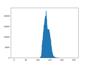
Illustration 2: histogram of original image

We will use Canny algorithm for edge detection as it is one of the most widely used algorithms and also suits our case. Canny implements Sobel operator to calculate image gradient. We must now determine an upper gradient threshold value Ʈu and a lower gradient threshold value Ʈl.

Ʈu – if gradient for a pixel lies above this value, it represents a strong edge

Ʈl  – if gradient for a pixel lies below this value, the pixel cannot lie on an edge

Canny classifies all pixels with gradient values between Ʈl and Ʈu as edges only if they are connected to strong edges. Assuming Canny as a system, our only task is to provide it with an input image and appropriate values for Ʈl and Ʈu. It will identify and output the edges for us.

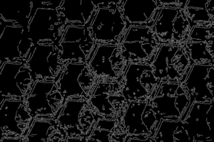
Illustration 3: edges on original with Ʈl as 10 and Ʈu  as 20

Without applying any transformation on the original image whose range is limited in a window of 40, determining Ʈl and Ʈu without generating false edges is cumbersome. With a small window, increasing or decreasing  either Ʈl or Ʈu by a single unit value has drastic impact on the edges detected. Without sacrificing hexagon edges, we obtained the best result on original with Ʈl   as 10 and  Ʈu as 20, as shown in illustration 3.

Though hexagon edges have been detected, many of them are connected with false and polluted edges.

Unsharp Masking

One way of increasing contrast locally near the edges without affecting uniform patches is through unsharp masking. We can get a brief gist from the following steps:

1. Unsharpen the original image by using Gaussian blur (convolution with Gaussian filter).
   The edges are blurred due to this. Now, if the absolute difference between blurred and original image is taken, only the blurred part in proximity of edges will come out as the difference.
2. We will take the weighted sum instead of the absolute difference.
   We have given a weight of 1.5 to the original image and -0.5 to the blurred image. We are inverting the blurred image through the negative 0.5 weight.

The following points explain how unsharp masking achieves edge sharpening:

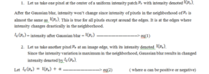
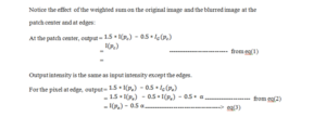
Now when a pixel lies at a whitish edge with blackish pixels on the other side, Gaussian blur results in calculated intensity lower than current edge pixel. Hence α will be negative.

When α is negative, eq(3) states that intensity at pixel increases by half the value of α. Hence intensity of pixels at the edges is upgraded, making them more whitish thereby enhancing contrast locally.

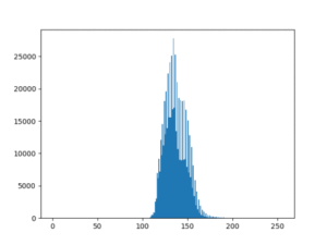
Illustration 4: histogram of original after unsharp mask

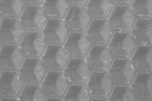
Illustration 5: unsharp masking on original image

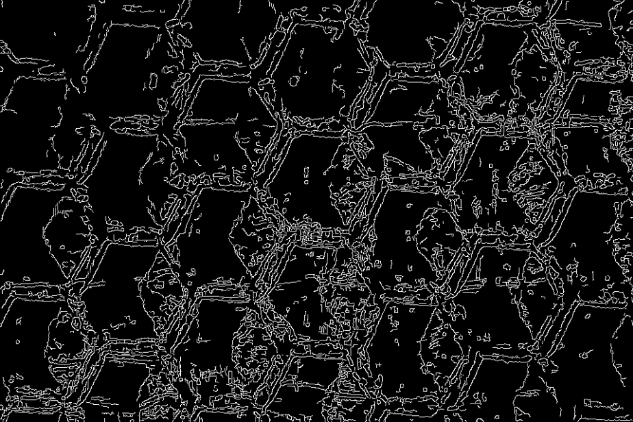
Illustration 6: edges in original after unsharp mask

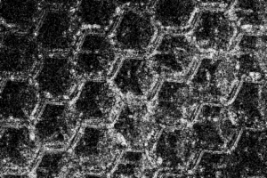
Illustration 7: bright pixels indicate the points where unsharp masking had an impact

Since unsharp mask does not change the intensity range, we can keep Ʈl and Ʈu the same as in the original image. But since it also sharpens the edge, it appears as if more polluted edges have emerged in comparison to illustration 3.

Gamma Transform

A common way to make dark pixels darker and keep bright pixels the same is gamma transform. The first step in gamma transform is to normalize the intensities.

Let us assume the following symbols:

• I(p) = intensity at pixel p
• In(p) = normalized intensity at pixel p
• Ig(p) = gamma transform of normalized intensity at pixel p

To normalize, we divide a given intensity by the maximum value possible of intensity range.

When values between 0 and 1 are squared, they diminish further. Normalization reduces intensities as follows:

• Values from [0, 85] ———————> reduced to —————-> [0, 0.33]
• Values from [86, 170] ———————> reduced to —————-> [0.34, 0.66]
• Values from [171, 255] ———————> reduced to —————-> [0.67, 1]

Squaring the normalized values brings in the following changes:

• [0, 0.33] ———————> squared to —————-> [0, 0.11]
• [0.34, 0.66] ———————> squared to —————-> [0.12, 0.44]
• [0.67, 0.90] ———————> squared to —————-> [0.45, 0.81]
• [0.91, 1] ———————> squared to —————-> [0.82, 1]

Now scaling back the reduced value completes the gamma transform:

• Values from [0, 85] ———————> transformed to —————-> [0, 28]
• Values from [86, 170] ———————> transformed to —————-> [29, 112]Values from [171, 255]  ———————> transformed to —————-> [113, 255]

As can be observed, dark pixel with values falling in 0 to 85 are gamma transformed to more darker intensities of 0 to 28. Brighter pixels closer to 255 remain almost the same, though slightly reduced. Hence gamma transform increases the contrast.

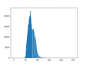
Illustration 8: histogram of original after gamma transform

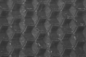
Illustration 9: gamma transform on original image

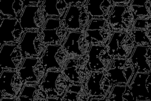
Illustration 10: edges on original after gamma transform with Ʈl  as 9 and Ʈu  as 19

Since the original intensity range itself was condensed, the output range after gamma transform did not have the expected effect. Instead of enhancing the contrast, it skewed all the pixel values towards 0. Hence the image in illustration 8 appears darker.

The intensity window has a size of approximately 50 which will again lead to the case of polluted edges being detected along with strong edges as depicted in illustration 9.

Histogram Equalization

Let us now introduce ourselves to one of the widely applied algorithm for visualization. Let us assume the following symbols:

• N = size of given image
• i = intensity in the range [0, 255]
• h(i) = number of pixels with intensity value as i

Note that,

By normalization, hn(i) is mapped to values between 0 and 1. Hence the normalized histogram represents probability distribution of intensities.

The next step to achieve equalization is to transform the probability of each intensity into cumulative probability. To equalize, let us assume the symbol:

• hcdf(i) = cumulative distribution function of probability at intensity i

Beginning at 0th intensity, we will go on accumulating the probabilities:

• hcdf(0) = hn(0)
• hcdf(1) = hcdf(0) + hn(1) = hn(0) + hn(1)
• hcdf(2) = hcdf(1) + hn(2) = hn(0) + hn(1) + hn(2)hcdf(255) = hcdf(254) + hn(255)  = hn(0) + hn(1) + hn(2) + ………….. + hn(255) = 1 ———–from eq(7)

As can be observed, any hcdf(i) lies between 0 and 1. The final step to equalize the distribution is to map values in range [0, 1] to range [0, 255]. Let us assume the following symbol:

• he(i) = output value of pixels with intensity i in the original image = 255*hcdf(i)

Let us observe the effect on the original image.

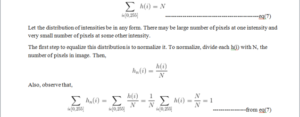
Illustration 11: histogram of original after histogram equalization

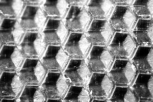
Illustration 12: histogram equalization of original image

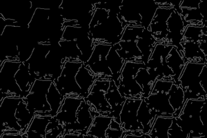
Illustration 13: edges on original after gamma transform with Ʈl   as 113 and Ʈu   as 150

Illustration 11 symbolizes the impact of histogram

equalization. The histogram has been completely stretched and the entire available range of intensity is covered. This makes it possible to clearly define the threshold for strong edges and thereby minimize the presence of polluted edges.

Note how Ʈl lies at 113 and Ʈu lies at 150, in comparison to the previous values of 13 and 20 respectively. Lot of strong edges lie above 150 and to ensure weaker hexagon edges get detected, we have decreased the upper threshold to 150, implying we now have a greater control varying the threshold values.

Conclusion: Combine The Three

As should have been apparent, combining all the three approaches provides us the best result. We applied histogram equalization first. Since the intensity is now distributed in its entire range, gamma transform can reach its maximum impact. Following it with unsharp masking will ensure the edges are further sharpened. Below are the illustrations of the result.

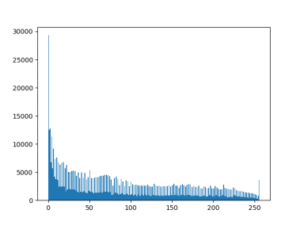
Illustration 14: histogram after combining the three approaches

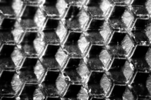
Illustration 15: contrast enhanced image by combining the three approaches

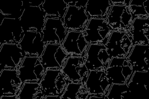
Illustration 16: edges detected after combining the three approaches with Ʈl   as 111 and Ʈu   as 194

Let us note how Ʈu has ascended to 195 and Ʈl is hovering at 111. At this point we have maximum control over varying the threshold values and can clearly distinguish strong and necessary edges from polluted edges.